
Beyond the Hype: Can Fine-Tuned LLMs Beat Custom Classifiers in Marketing Campaign Prediction?
Our custom-built machine learning models have served us well, becoming the reliable champions for our classification needs. But a new challenger has emerged. The rapid advance of Large Language Models (LLMs) raises a compelling question that we couldn’t ignore:
Can the vast, pre-trained knowledge of an LLM actually beat a specialized model on its own turf?
To find a definitive answer, we launched an in-house deep dive with three core objectives:
1. The Testbed: A Realistic Business Problem. First, we needed a meaningful challenge. We chose a marketing campaign classification task, using our own synthetically generated datasets to predict success as Underperforming, Average Performing, or Overperforming.
2. The Core Question: A Head-to-Head Showdown. Our primary goal was to definitively determine if a fine-tuned LLM could match or exceed the performance of our best internal classifiers on this specific task.
3. The Strategic Goal: Building In-House Capability. Beyond this single experiment, we aimed to develop our team’s practical expertise in fine-tuning and deploying LLMs by systematically exploring different workflows and their trade-offs.
This blog post details that journey. We will walk you through our methodology, from our multi-pronged fine-tuning strategy to a final showdown between our internal champion and the chosen LLM challengers: Gemini, Gemma, and Qwen.
The Quest: Our Three-Pronged Experimental Strategy
A core objective was to develop a versatile, in-house capability for LLM fine-tuning. To achieve this, we deliberately explored three distinct workflows, each representing a different point on the spectrum of control and complexity:
| Workflow | Model | Approach | Key Characteristic |
|---|---|---|---|
| 1. The Managed Expressway | Gemini 2.5 Flash-Lite | Fully Managed (Vertex AI) | Low-overhead and serverless, but a “black box” with limited control. |
| 2. The Custom Highway | Gemma3-1b-it | Custom Cloud Training (Vertex AI) | A middle ground offering more control with the scalability of the cloud. |
| 3. The Hands-On Workshop | Qwen3-4b-base | Local Training (Local GPU) | Maximum control and deep architectural customization. |
This multi-faceted approach enabled us to build robust internal knowledge for future LLM projects while systematically testing our core hypothesis.
The Proving Ground: Our Datasets
To ensure a controlled and repeatable experiment, our analysis was performed on a suite of synthetically generated datasets, all created by our in-house ground-truth graph generator, a custom-built system designed specifically to simulate realistic marketing and media performance dynamics. By generating data with known underlying relationships, this system allows us to test AI models in a fully transparent, controlled environment while preserving the complexity of real-world campaign dynamics.
Each campaign in our dataset is described by five text-based features, designed to mimic a real-world marketing brief:
- Audience: A qualitative description of the target consumer segment, including their values and interests.
- Brand: The market positioning, values, and perceived credibility of the brand.
- Creative: The tone, messaging style, and persuasive approach of the ad content.
- Platform: The advertising platform where the campaign runs (e.g., Amazon, TikTok), which implies user intent and context.
- Geography: The geographic region being targeted as a series of zip-codes, providing demographic and market signals.
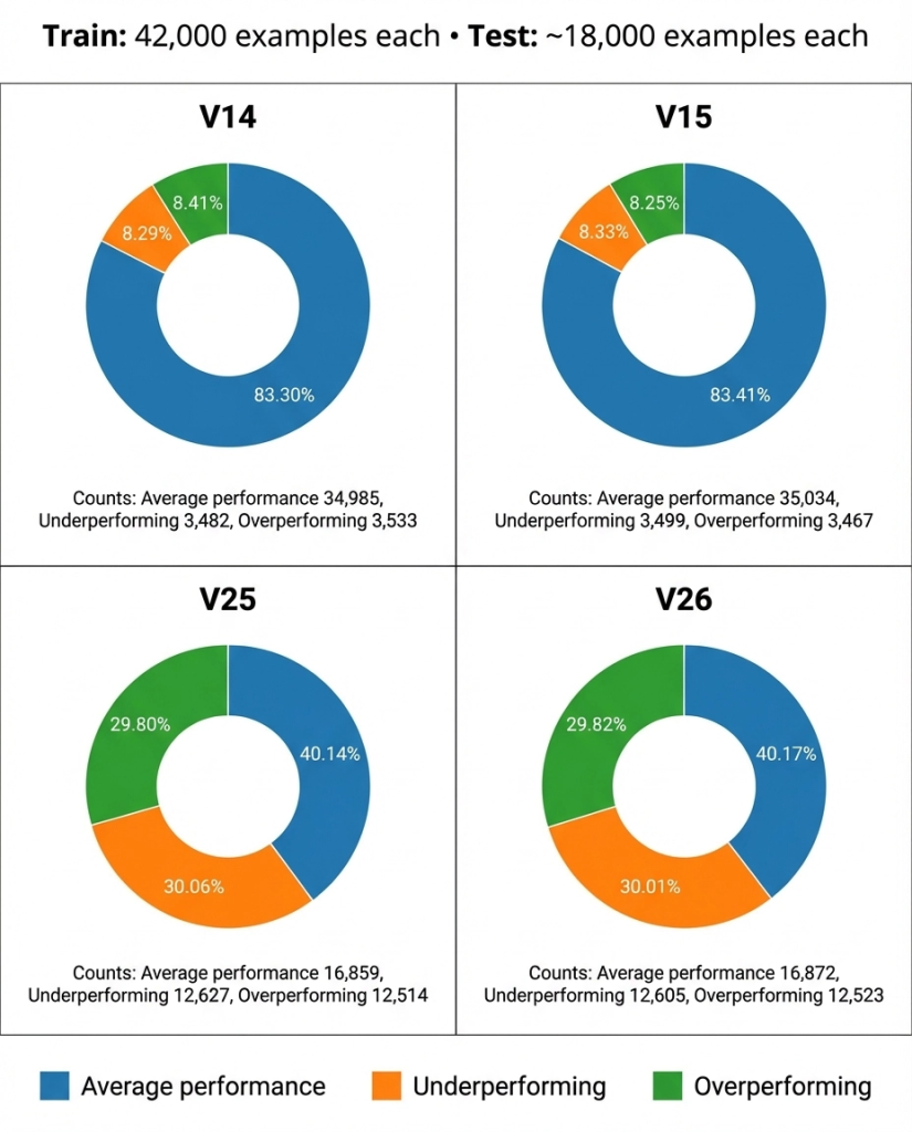
With this setup, the model’s task was to predict campaign success. All dataset versions contain 42,000 training examples but were designed with two distinct class distributions to test the models under different conditions:
- Highly Imbalanced Sets (
V14,V15): These datasets present a significant class imbalance challenge where theAverage Performingclass is overwhelmingly dominant. This setup was specifically designed to see if the models would fall into the “average trap.” - Balanced Sets (
V25,V26): In contrast, these datasets are far more balanced, with the three classes distributed much more evenly. These test the model’s ability to distinguish between classes when no single class is an easy default.
The chart below provides a clear visual breakdown of this intentional variation, illustrating the stark difference in class distribution across our four primary training datasets:
Synthetic Dataset Class Distributions’ Summary
Finally, a crucial component of our methodology was the strict separation of respective test datasets containing approximately 18,000 entries each. Unlike the training sets, the true labels for this test data were never exposed to our team. Instead, evaluation was conducted exclusively through a blind API service. This protocol was essential to prevent any form of data leakage or unconscious bias from influencing our model development and hyperparameter tuning, ensuring a truly honest assessment of each model’s performance.
Round 1: The Managed Approach with Gemini
For the first leg of our journey, we turned to Google’s fully managed, serverless pipeline on Vertex AI to fine-tune the Gemini model. This approach represented the “path of least resistance,” allowing us to establish a performance baseline with a state-of-the-art model using a streamlined, integrated platform with minimal operational overhead.
The Setup: LoRA, a “Black Box” with Limited Levers
It’s critical to understand that the supervised fine-tuning for Gemini models on Vertex AI uses a Parameter-Efficient Fine-Tuning (PEFT) method called LoRA, which stands for Low-Rank Adaptation.
Instead of retraining all the billions of parameters in the model (a process known as full fine-tuning), LoRA freezes the vast majority of the base model’s weights.
It then injects small, trainable modules called “adapters” into the model’s architecture.
The fine-tuning process only updates the parameters within these lightweight adapters, which can reduce the number of trainable parameters by up to 10,000 times.
This LoRA-based methodology has several profound implications:
- Efficiency and Cost: It dramatically reduces the computational cost, memory requirements, and time needed for fine-tuning.
- Portability: The output of the process is not a new multi-billion parameter model, but a small adapter file (typically just a few megabytes) that is “placed on top” of the base model during inference.
- Preservation of Knowledge: Because the core model is frozen, this method prevents “catastrophic forgetting,” where a model can lose its powerful, general-purpose knowledge during specialization.
However, for our experiment, the most important implication is that it limits the scope of customization. We are not changing the core model; we are only training the adapters. The primary levers available in the Vertex AI service are dials to control this adapter-based training:
- Training Steps: The total number of steps the model trains for (which we map from epochs).
- Learning Rate Multiplier: A multiplier applied to a recommended, pre-tested learning rate for the adapter.
- Adapter Size (Rank): This directly controls the capacity (the number of trainable parameters) of the LoRA matrices. A larger rank gives the adapter more power to learn the new task but also increases its size. Common options are powers of 2 (e.g., 4, 8, 16).
Experiments and Results: Turning the Dials on the Black Box
We ran a series of experiments across our datasets to see if we could find a combination of these limited hyperparameters that would yield competitive performance. The table below summarizes our key runs and their results.
Table 1: Gemini Flash Lite Performance Across All Datasets
| Dataset | Model | Overall F1 | Negative F1 | Average F1 | Positive F1 | Epochs | LR Multiplier | Adapter Size |
|---|---|---|---|---|---|---|---|---|
| V15 | Internal (Best) | 0.9280 | 0.9215 | 0.9807 | 0.8818 | N/A | N/A | N/A |
| V15 | Gemini (Baseline) | 0.2693 | 0.1249 | 0.5350 | 0.1480 | 0 | N/A | N/A |
| V15 | Gemini (Fine-Tuned) | 0.3381 | 0.0998 | 0.8333 | 0.0812 | 5 | 1 | 4 |
| V25 | Internal (Best) | 0.8947 | 0.9125 | 0.8595 | 0.9122 | N/A | N/A | N/A |
| V25 | Gemini (Fine-Tuned) | 0.3329 | 0.2928 | 0.3974 | 0.3086 | 10 | 2 | 16 |
| V26 | Internal (Best) | 0.8884 | 0.9113 | 0.8526 | 0.9014 | N/A | N/A | N/A |
| V26 | Gemini (Fine-Tuned) | 0.3335 | 0.2912 | 0.4019 | 0.3074 | 10 | 2 | 16 |
Dissecting the Performance: A Look at Controlled Experiments
To understand if this performance ceiling could be breached, we conducted several controlled experiments to isolate the impact of different variables.
Model Scale
We first questioned if a larger model would perform better. Table 2 compares gemini-2.5-flash-lite with the slightly larger gemini-2.5-flash, keeping all other hyperparameters identical.
Table 2: Gemini Model Comparison (Flash Lite vs. Flash)
| Model Name | Overall F1 | Negative F1 | Average F1 | Positive F1 | Epochs | LR Multiplier | Adapter Size | Sys Prompt |
|---|---|---|---|---|---|---|---|---|
gemini-2.5-flash-lite | 0.3254 | 0.0728 | 0.8037 | 0.0996 | 5 | 1 | Four | 2 |
gemini-2.5-flash | 0.3381 | 0.0998 | 0.8333 | 0.0812 | 5 | 1 | Four | 2 |
The larger gemini-2.5-flash model provided a marginal improvement in the Overall F1-score. This suggests that while scale can help slightly, it does not fundamentally solve the architectural challenges of this workflow.
Hyperparameter Tuning
Next, we analyzed the impact of training duration and learning rate. Table 3 compares our two primary training configurations.
Table 3: Gemini Flash Lite Epoch and LRM Comparison
| Epochs | LR Multiplier | Dataset | Overall F1 | Negative F1 | Average F1 | Positive F1 |
|---|---|---|---|---|---|---|
| 5 | 1 | V15 | 0.3293 | 0.0842 | 0.8068 | 0.0969 |
| 10 | 2 | V25 | 0.3329 | 0.2928 | 0.3974 | 0.3086 |
| 10 | 2 | V26 | 0.3335 | 0.2912 | 0.4019 | 0.3074 |
Here, we see a crucial finding. The runs with 10 Epochs and a Learning Rate Multiplier of 2 (on V25 and V26) yielded significantly better F1-scores on the minority “Negative” and “Positive” classes compared to the 5-epoch run. This indicates that more extensive training helped the model learn more about the rare classes, but it still wasn’t enough to lift the overall performance to a competitive level.
Our experiments with Adapter Size and System Prompts showed that these parameters had a negligible impact on performance. Whether using an adapter size of “Four” or “Sixteen,” or using prompts with text versus integer labels, the results remained consistently low, confirming that the bottleneck was not these specific settings.
System Prompt Strategy
Next we needed to control for was the prompt itself. Was the model’s poor performance simply due to a misunderstanding of the task’s objective? To isolate this, we designed and tested distinct prompt strategies that framed the classification problem in fundamentally different ways:
- Persona-Based Reasoning (System Prompt 1): This prompt instructed the model to assume the role of a senior marketing expert and use its vast pre-trained knowledge of consumer behavior and brand strategy to make a qualitative judgment.
- Rule-Based Classification (System Prompts 2 & 3): These prompts explicitly described the quantitative, rule-based logic used to generate our synthetic data. They instructed the model to ignore qualitative interpretation and instead focus on tallying the positive and negative relationships between features to arrive at a classification, outputting either a text label (Prompt 2) or an integer label (Prompt 3).
The results of this test were immediate and revealing.
SYSTEM_PROMPT = {
    # System prompt 1: Assuming the role of a marketing professional and relying on the models' historical data
    1: """
### Role
You are a senior marketing campaign manager with deep experience designing and evaluating advertising campaigns across digital platforms.

You understand:
- Brand positioning, perceived value, and product–market fit
- Consumer behavior, lifestyle signals, and purchasing psychology
- Audience–channel alignment and creative effectiveness
- How targeting, creative tone, and platform context influence campaign outcomes

### Task
Your task is to accurately predict the expected performance of an advertising campaign based on the provided features. Using your professional judgment, classify the campaign’s expected performance into exactly ONE of the following categories.

### Input Field Definitions
- **Audience**: A qualitative description of the target consumer segment, including lifestyle habits, behavioral tendencies, interests, and personal values. This input should be interpreted as an indicator of audience–product and audience–platform fit.
- **Brand**: A description of the brand’s positioning, values, credibility, and market perception. This input reflects brand strength, authority, and alignment with the intended audience and campaign objectives.
- **Creative description**: The tone, messaging style, emotional intensity, and persuasive approach of the campaign’s creative content. This input should be evaluated for clarity, relevance, resonance with the audience, and consistency with the brand.
- **Geolocation**: A list of geographic targeting identifiers (e.g., ZIP codes) indicating where the campaign will be shown. This input provides contextual signals such as market characteristics, demographic tendencies, and historical regional performance.
- **Platform**: The advertising or commerce platform where the campaign will run (e.g., Amazon). This input represents platform-specific user intent, audience behavior, format constraints, and historical performance patterns.

### Output Label Definitions
- **Overperforming**: Based on historical data, more than 70% of campaigns with similar input features achieved a positive return on investment (ROI).
- **Average performance**: Based on historical data, between 40% and 70% of campaigns with similar input features achieved a positive return on investment (ROI).
- **Underperforming**: Based on historical data, fewer than 40% of campaigns with similar input features achieved a positive return on investment (ROI).

### Instructions & Output Format
Your output must be a single string, one of:
- Overperforming
- Average performance
- Underperforming

Do not include explanations, reasoning, or any additional text.

### Campaign to Classify
Audience: {{audience}}
Brand: {{brand}}
Creative description: {{creative}}
Platform: {{platform}}
Geography: {{geography}}

### Classification Output
Label: {{label}}
""",
    # System prompt 2: Reverse engineering the methodology used to assign labels via the graph generator
    2: """
### Role
You are a classifier tasked to annotate marketing campaigns of a given setup as Overperforming, Underperforming or Average performance.

### Task
You are provided with examples of synthetic data examples that were generated based on pairwise relationships (positive, negative or neutral) between the different attributes of the campaign settings. If an example has many positive pairwise relationships it is considered overperforming and if it has many negative relationships it is considered underperforming. All attributes are considered of equal importance so it is only the amount of pairwise relationships that determines the overall campaign performance, not their quality.

### Instructions & Output Format
Your output must be a single string, one of:
- Overperforming
- Average performance
- Underperforming

Do not include explanations, reasoning, or any additional text.

### Campaign to Classify
Audience: {{audience}}
Brand: {{brand}}
Creative description: {{creative}}
Platform: {{platform}}
Geography: {{geography}}

### Classification Output
Label: {{label}}
""",
    # System prompt 3: Reverse engineering the methodology used to assign labels via the graph generator using integer output labels
    3: """
### Role
You are a classifier tasked to annotate marketing campaigns of a given setup as Overperforming, Underperforming or Average performance.

### Task
Classify the campaign by tallying the pairwise relationships between all attributes, treating every attribute as mathematically equal in importance. Calculate the net balance of these interactions: a majority of positive relationships defines the campaign as 2 (overperforming), while a majority of negative relationships defines it as 0 (underperforming). If the relationships are predominantly neutral or the positive and negative counts are equal, classify it as 1 (average performance). Your decision must be based strictly on the quantity of relationship types, ignoring the qualitative nature of the descriptions or the perceived importance of any single setting.

### Instructions & Output Format
Your output must be a single integer, one of:
- 0 (for Underperforming)
- 1 (for Average performance)
- 2 (for Overperforming)

Do not include explanations, reasoning, or any additional text.

### Campaign to Classify
Audience: {{audience}}
Brand: {{brand}}
Creative description: {{creative}}
Platform: {{platform}}
Geography: {{geography}}

### Classification Output
Label: {{integer label}}
""",
}
The persona-based approach (System Prompt 1) yielded extremely poor results and was quickly discarded from formal evaluation. Our hypothesis is that instructing the model to rely on its general, pre-trained “marketing knowledge” created a direct conflict with the specific, mathematical classification objective of our synthetic dataset. The model was trying to solve the wrong problem.
Table 4: Gemini System Prompt Comparison
| Sys Prompt | Overall F1 | Negative F1 | Average F1 | Positive F1 | Epochs | LR Multiplier | Adapter Size |
|---|---|---|---|---|---|---|---|
| 2 | 0.3381 | 0.0998 | 0.8333 | 0.0812 | 5 | 1 | Four |
| 3 | 0.3323 | 0.0897 | 0.8247 | 0.0824 | 5 | 1 | Four |
As shown in Table 4, the two rule-based prompts performed almost identically, confirming that the model understood the task equally well with either a text or integer output format. This confirmed that the prompt strategy was not the bottleneck; the performance ceiling was due to more fundamental architectural limitations of the managed workflow.
Analysis: Hamstrung by the LoRA and Generative Combination
The results table paints a clear and consistent picture across all datasets. Despite our experimentation with hyperparameters—increasing epochs, raising the learning rate multiplier, and using a larger adapter size and even changing the model to the pro and lite versions—we saw no significant breakthrough. Here are the key findings and the perceived reasons behind them.
1. Internal Models Reign Supreme
The most immediate takeaway is the stark performance gap. On our high-performing datasets (V15, V25, and V26), our internal models achieve outstanding Overall F1-scores approaching or exceeding 0.90. The fine-tuned Gemini model, in contrast, struggles to score above 0.34. This highlights the enduring power of a specialized classifier that has been purpose-built and refined for a specific task.
2. The LLM Falls into the “Average” Trap
The class-level F1-scores reveal the core issue. Across all experiments, the Gemini model shows a strong bias toward the majority “Average” class. On dataset V15, for example, it achieves a respectable F1-score of around 0.83 for “Average”, but performs extremely poorly on the minority classes, with scores falling below 0.10.
This behaviour is a classic symptom of learning on imbalanced data. Because the model is trained to generate a text label, it quickly learns that predicting the most common class is the safest way to minimize its training loss. Within the constraints of LoRA-based fine-tuning, the model tends to rely on this shortcut rather than learning the more subtle patterns that distinguish the minority classes.
It’s possible that training for many more epochs could gradually improve these results. However, doing so would significantly increase training time and cost, and given the large performance gap compared to our internal models, it was not a trade-off we considered worthwhile.
3. Specialization Wins at the Edges
In stark contrast, our internal models demonstrate robust and balanced performance. They post high F1-scores not only for the majority class but also for the difficult “Negative” and “Positive” classes. This shows their ability to learn the nuanced features that distinguish these minority groups, a capability that is essential for providing real business value.
4. Architecture, Not Just Parameters, Is Key
The tweaks to LoRA hyperparameters were not enough to bridge the fundamental performance gap. The issue is architectural. The combination of a purely generative training objective (producing a text label) and the inherent limitations of a “black box” PEFT service proved to be an insurmountable obstacle. The approach, while flexible, is less efficient for this highly specific classification task than a traditional discriminative model explicitly designed to optimize a classification objective (like cross-entropy loss).
Conclusion for the Gemini Workflow
Our experiment with the fully managed Gemini pipeline was an invaluable exercise. It provided an accelerated path to establish a performance baseline and was instrumental in building our team’s initial LLM capabilities. However, for our specific, highly imbalanced classification task, it is not a viable replacement for our existing, specialized models.
The key lesson is that while LLMs are incredibly powerful, they are not a universal solution. The managed, “black box” nature of the Gemini fine-tuning workflow, which treats classification as a text-generation task, proved to be a fundamental architectural mismatch for our needs. This approach prevented the model from effectively learning the nuanced features of the minority classes—a problem that could not be solved by simply adjusting standard hyperparameters like learning rate, model size, or prompt strategy.
Round 2: The Custom Highway with Gemma
After hitting a performance ceiling with the managed Gemini pipeline, it was clear we needed more control. The “black box” nature of the service, combined with its generative training objective, was preventing us from tackling the core issue of class imbalance.
For our second round, we moved to the “Custom Highway”: fine-tuning Gemma, Google’s family of open-weights models, using Vertex AI Custom Training. This approach represents the perfect middle ground, granting us the granular control of a custom training script while still leveraging the scalability and convenience of cloud infrastructure.
The Setup: Full Fine-tuning with strategic layer freezing
A critical departure from the Gemini workflow was abandoning the constraints of PEFT/LoRA. Instead, we opted for full fine-tuning, where the model’s core weights are made trainable. This custom approach unlocked a new level of control, giving us direct access to the core mechanics of the training process. The “levers” at our disposal were no longer just dials on a managed service but fundamental architectural and hyperparameter choices:
- Epochs: The total number of times the model sees the entire training dataset. We now had direct control over the full training cycle, giving us a clearer understanding of the risk of under-training versus overfitting.
- Learning Rate: This determines the size of the adjustments made to the model’s weights. We could now set the absolute learning rate (e.g.,
2e-4,1e-5), giving us far more precision than the simple “multiplier” available in the managed Gemini service. - Layer Freezing Strategy: This became our primary architectural lever for regularization. To manage the power of full fine-tuning and prevent catastrophic forgetting, we employed this strategic technique. By freezing the bottom 14 layers, we anchored the model to its powerful, pre-trained foundation of general language understanding while allowing the upper, more task-specific layers full flexibility to adapt.
- Inference-Time Architecture (
LogitsProcessor): Our most powerful adaptation was a change to the model’s behavior at the moment of inference. This customLogitsProcessoris a function that intercepts the model’s output and works as follows:- Intercept: After the model processes the input prompt and is ready to generate an output, the
LogitsProcessorsteps in. - Filter: It examines the logits—the raw probability scores for every token in the model’s vocabulary.
- Constrain: It programmatically sets the probability of all tokens to zero, except for the specific tokens corresponding to our allowed class labels: “0”, “1”, and “2”.
- Decide: The model is thus forced to choose from this tiny, pre-approved set of tokens.
- Intercept: After the model processes the input prompt and is ready to generate an output, the
This final technique is a game-changer. It effectively transforms the generative model into a true classifier at the moment of prediction. Instead of learning to generate the text of a label, it learns to assign the highest probability to the single correct token from a fixed list, directly addressing the architectural flaw we identified in the Gemini workflow.
Experiments and Results: The Journey to Parity
With this powerful new tool in our arsenal, we began a methodical search for the best configuration. Arriving at the optimal result wasn’t a single step but a journey of experimentation with key hyperparameters.
Hyperparameter Exploration: Finding the “Sweet Spot”
The table below details our hyperparameter exploration on the V15 dataset. It illustrates the journey from an unusable baseline, through under-training and over-training, to finding the optimal “sweet spot” for epochs and learning rate that allowed Gemma to rival our best internal model.
Table 5: Gemma Hyperparameter Exploration (Dataset V15)
| Model | Overall F1 | Negative F1 | Average F1 | Positive F1 | Epochs | LR |
|---|---|---|---|---|---|---|
| Internal (Best) | 0.9280 | 0.9215 | 0.9807 | 0.8818 | N/A | N/A |
| Gemma 3.1B (Over-trained) | 0.4440 | 0.3590 | 0.6035 | 0.3693 | 20 | 1e-5 |
| Gemma 3.1B (Optimal) | 0.9015 | 0.9091 | 0.9742 | 0.8213 | 8 | 2e-4 |
| Gemma 3.1B (Under-trained) | 0.5943 | 0.5206 | 0.8070 | 0.4553 | 3 | 1e-5 |
| Gemma 3.1B (Baseline) | 0.0523 | 0.0000 | 0.0001 | 0.1569 | 0 | N/A |
This exploration reveals several crucial insights:
- Fine-Tuning is Essential, But Not Foolproof: The baseline Gemma model was completely ineffective. Just three epochs of fine-tuning yielded a massive performance jump. However, the run with 20 epochs shows a classic case of overfitting, where the model begins to memorize the training data and performance collapses.
- The Optimal Configuration: The run with 8 epochs and a learning rate of 2e-4 proved to be the sweet spot. With an Overall F1-score of ~0.90, this fine-tuned Gemma model achieved performance remarkably close to our best internal model (0.9280). Most importantly, the class-level F1-scores are strong and balanced, demonstrating that our
LogitsProcessorhad successfully forced the model to learn the minority classes.
Architectural Choices Vindicated
This success wasn’t just about hyperparameters. We also validated two other key architectural choices.
Table 6: Layer Freezing & Model Scaling Comparison
| Dataset | Model | Note | Overall F1 | Negative F1 | Average F1 | Positive F1 |
|---|---|---|---|---|---|---|
| V14 | Gemma 3.1B | Default (14 Layers Frozen) | 0.3154 | 0.0039 | 0.9043 | 0.0379 |
| V14 | Gemma 3.1B | Fewer (8 Layers Frozen) | 0.3039 | 0.0013 | 0.9103 | 0.0000 |
| — | — | — | — | — | — | — |
| V15 | Gemma 3.1B (Optimal) | 0.9015 | 0.9091 | 0.9742 | 0.8213 | |
| V15 | Gemma 3.4B FT | Larger Model | 0.8663 | 0.8739 | 0.9659 | 0.7592 |
As shown in Table 6, our default strategy of freezing the bottom 14 layers of the Gemma model proved slightly superior to freezing fewer layers, suggesting it provides a valuable regularizing effect. Furthermore, we found that a larger Gemma 4B model did not outperform our optimal 1.1B model. This is a powerful reminder that for a given task, there is a “sweet spot” for model size, and more parameters are not always the answer.
Table 7: Gemma Performance Across All Datasets
| Dataset | Model Type | Overall F1 | Negative F1 | Average F1 | Positive F1 | Epochs | LR | Sys Prompt |
|---|---|---|---|---|---|---|---|---|
| V14 | Internal (Best) | 0.4059 | 0.2225 | 0.8191 | 0.1760 | N/A | N/A | N/A |
| V14 | Gemma (FT, Default Frozen) | 0.3154 | 0.0039 | 0.9043 | 0.0379 | 8 | 0.0002 | 3 |
| V14 | Gemma (FT, Fewer Frozen) | 0.3039 | 0.0013 | 0.9103 | 0.0000 | 8 | 0.0002 | 3 |
| — | — | — | — | — | — | — | — | — |
| V15 | Internal (Best) | 0.9280 | 0.9215 | 0.9807 | 0.8818 | N/A | N/A | N/A |
| V15 | Gemma (Baseline) | 0.0523 | 0.0000 | 0.0001 | 0.1569 | 0 | N/A | 3 |
| V15 | Gemma (FT, Optimal) | 0.9015 | 0.9091 | 0.9742 | 0.8213 | 8 | 0.0002 | 3 |
| — | — | — | — | — | — | — | — | — |
| V25 | Internal (Best) | 0.8947 | 0.9125 | 0.8595 | 0.9122 | N/A | N/A | N/A |
| V25 | Gemma (FT, Default Frozen) | 0.8527 | 0.9052 | 0.8303 | 0.8226 | 8 | 0.0002 | 3 |
| — | — | — | — | — | — | — | — | — |
| V26 | Internal (Best) | 0.8884 | 0.9113 | 0.8526 | 0.9014 | N/A | N/A | N/A |
| V26 | Gemma (FT, Default Frozen) | 0.8845 | 0.9059 | 0.8470 | 0.9005 | 8 | 0.0002 | 3 |
Bonus: What Did the LLM Actually Learn?
After achieving parity, we wanted to understand what the fine-tuned LLM had learned. We conducted a feature ablation study, re-training our best Gemma model multiple times while removing one feature at a time. A larger drop in performance indicates a more important feature.
Table 8: Gemma Feature Importance (Dataset V15)
| Feature Removed | Overall F1 | Negative F1 | Average F1 | Positive F1 | Performance Drop |
|---|---|---|---|---|---|
| Brand | 0.8449 | 0.8067 | 0.9604 | 0.7677 | 0.0647 |
| Platform | 0.8681 | 0.8673 | 0.9627 | 0.7742 | 0.0416 |
| Creative | 0.8719 | 0.8617 | 0.9641 | 0.7898 | 0.0378 |
| Audience | 0.8798 | 0.8622 | 0.9668 | 0.8105 | 0.0299 |
| Geography | 0.9053 | 0.9098 | 0.9745 | 0.8317 | 0.0044 |
| — | — | — | — | — | — |
| None (Full Model) | 0.9097 | 0.9099 | 0.9753 | 0.8439 | 0.0000 |
The results are remarkably clear and align with marketing intuition: Brand, Platform, and Creative are the most critical predictors of campaign success. This analysis provides invaluable insight, confirming that the LLM is learning logical, interpretable patterns and can be used not just for prediction, but for generating deep, actionable business insights.
Analysis: How Control and Architecture Led to a Breakthrough
The Gemma results stand in stark contrast to our experience with the managed Gemini pipeline. The success story here is not just about the final numbers but about how we achieved them.
1. Parity Achieved: From Unusable to Unbeatable
This is the headline finding. The baseline Gemma model was completely unusable, with an F1-score near zero. However, after methodical fine-tuning, its performance skyrocketed to ~0.90, virtually matching the performance of our highly specialized internal model (~0.93). This is a monumental result, demonstrating that with the right approach, a fine-tuned open-weights LLM can indeed close the gap and compete with a purpose-built classifier.
2. Escaping the “Average” Trap: The LogitsProcessor as a Game-Changer
The catastrophic failure on minority classes we saw with Gemini is gone. Table 5 shows that the optimized Gemma model’s F1-scores are strong and balanced across all classes, including the difficult “Negative” (0.9091) and “Positive” (0.8213) categories. This directly validates our hypothesis: the architectural choice to use a LogitsProcessor was the silver bullet. It prevented the model from defaulting to the majority class and forced it to learn the distinguishing features of the minority classes, a feat the generative-only Gemini workflow could not accomplish.
3. Architectural Choices Are Vindicated
This successful tuning process proves that the right architecture is more important than just turning dials. The control afforded by the custom pipeline was fundamental.
- Full Fine-Tuning over PEFT: The decision to use full fine-tuning (with strategic layer freezing) instead of the more constrained LoRA method gave the model the necessary capacity to learn our task.
- The Power of the
LogitsProcessor: This allowed us to reshape the model’s behavior at its core, turning it into a true classifier.
These architectural choices created a sound foundation where hyperparameter tuning could have a meaningful impact, unlike in the Gemini workflow where tuning was like trying to polish a flawed design.
Conclusion for the Gemma Workflow
The Gemma experiment was a resounding success. It proved that by taking a “middle ground” approach—combining the flexibility of an open-weights model, the power of full fine-tuning with strategic layer freezing, and the architectural rigor of a LogitsProcessor—we can build LLM-based solutions that are truly competitive with established, specialized models. This workflow has become a cornerstone of our internal LLM capability, providing a powerful and versatile template for future projects.
Round 3: The Hands-On Workshop with Qwen
After achieving parity with Gemma, we took the final step in our journey: descending into the “Hands-On Workshop.” The goal of this round was to take ultimate control of the training process by setting up a local environment on a Google Cloud VM to fine-tune Qwen3-4B-Base, an open-weights model.
It is important to note that this workflow was the least explored in terms of exhaustive hyperparameter optimization. Our primary goal here was to establish a proof of concept: could we successfully fine-tune a different open-weights model in a fully custom environment and test our most radical architectural idea yet?
The Setup: A Code Walkthrough of Surgical Precision
The local workshop environment gave us unparalleled control over the entire training stack. Let’s walk through the key implementation details in our Python scripts to see how this was achieved.
Step 1: Efficient PEFT with Unsloth (model.py)
Interestingly, this workflow marked a return to a Parameter-Efficient Fine-Tuning (PEFT) method, specifically LoRA. However, this was fully transparent and controllable, unlike the managed Gemini service. We used the unsloth library, which provides a highly optimized implementation of LoRA.
As seen in model.py, we load the model with 4-bit quantization and prepare it for LoRA training with a single, efficient command:
# From model.py
model, tokenizer = FastLanguageModel.from_pretrained(
    model_name = model_id,
    max_seq_length = max_seq_length,
    dtype = dtype,
    load_in_4bit =True,
)
This embraces PEFT as a deliberate choice for efficiency on a single GPU, not as a service-imposed constraint.
Step 2: Direct Architectural Modification
Our most powerful adaptation was performing “surgery” on the model’s architecture. Before applying the LoRA adapters, we fundamentally reshaped the LLM into a direct classifier. The prepare_model_for_classification_head() function in model.py executes this surgical strike.
# From model.py
def prepare_model_for_classification_head(model, num_classes=3):# Get the lm_head's weights
    lm_head = model.get_output_embeddings()# Trim the vocabulary to the number of classes
    trimmed_lm_head_weight = lm_head.weight[:num_classes, :]# Create a new head with the trimmed weights
    new_lm_head = torch.nn.Linear(
        in_features=trimmed_lm_head_weight.shape[1],
        out_features=trimmed_lm_head_weight.shape[0],
        bias=False
    )
    new_lm_head.weight.data = trimmed_lm_head_weight# Set the model's new head
    model.set_output_embeddings(new_lm_head)
This code trims the model’s final output layer (lm_head) from tens of thousands of potential tokens down to just three outputs. The model is no longer physically capable of generating text beyond our class labels. It is now, by its very architecture, a true classification model.
Step 3: Training with a Custom Data Collator (trainer.py)
With a classification head in place, our trainer.py script uses a custom DataCollatorForLastTokenLM. Its job is to ensure that during training, the loss is calculated only on the model’s prediction for the final token, forcing the model to focus all its learning capacity on the classification task.
Step 4: Post-Inference Logic with Confidence Boosting (evaluator.py)
Finally, to combat the class imbalance we knew would still exist in the model’s learned weights, our evaluator.py script implements a post-processing --boost flag.
# From evaluator.py
if args.boost:# Manually increase logits for minority classes
    logits[:,0] = logits[:,0] *2.5
    logits[:,2] = logits[:,2] *2.5
This code intercepts the raw logits from the model’s output and multiplies the scores for the minority “Underperforming” (0) and “Overperforming” (2) classes. This artificially “boosts” their chances of being selected before the final probabilities are calculated, giving us a direct tool to counteract the model’s learned biases.
Experiments and Results: A Powerful Technique with Mixed Results
As this was a proof of concept, our experimentation was focused on these new architectural changes. Table 9 shows the progression on the V15 dataset as we applied each new technique.
Table 9: Qwen Architectural Progression (Dataset V15)
| Model | Note | Overall F1 | Negative F1 | Average F1 | Positive F1 |
|---|---|---|---|---|---|
| Internal (Best) | 0.9280 | 0.9215 | 0.9807 | 0.8818 | |
| Qwen3 (Baseline) | 0.2470 | 0.1453 | 0.4902 | 0.1056 | |
| Qwen3 (Fine-Tuned) | Trimmed LM Head | 0.4468 | 0.1919 | 0.8824 | 0.2661 |
| Qwen3 (Fine-Tuned) | + Boosted | 0.4668 | 0.2412 | 0.8716 | 0.2876 |
To confirm if these results were consistent, we ran our best configuration (fine-tuned with boosting) across our other high-quality datasets.
Table 10: Qwen Performance Across All Datasets
| Dataset | Model Type | Note | Overall F1 | Negative F1 | Average F1 | Positive F1 |
|---|---|---|---|---|---|---|
| V15 | Internal (Best) | 0.9280 | 0.9215 | 0.9807 | 0.8818 | |
| V15 | Qwen3 (FT) | + Boosted | 0.4668 | 0.2412 | 0.8716 | 0.2876 |
| — | — | — | — | — | — | — |
| V25 | Internal (Best) | 0.8947 | 0.9125 | 0.8595 | 0.9122 | |
| V25 | Qwen3 (FT) | + Boosted | 0.3480 | 0.2380 | 0.5733 | 0.2327 |
| — | — | — | — | — | — | — |
| V26 | Internal (Best) | 0.8884 | 0.9113 | 0.8526 | 0.9014 | |
| V26 | Qwen3 (FT) | + Boosted | 0.3731 | 0.2907 | 0.5766 | 0.2519 |
Analysis: An Insightful Technique That Underperformed
The cross-dataset results tell a clear and consistent story.
1. Architectural Promise, But Performance Lags: The direct classification approach showed significant promise in Table 9, far exceeding the baseline. However, Table 10 shows that even our best configuration consistently underperformed against both our internal models and the optimized Gemma pipeline, often by a margin of 0.50 or more on the Overall F1 score.
2. Boosting Helps, But It’s a Patch, Not a Fix: The confidence boosting technique consistently provided a small but measurable improvement (as seen in Table 9). This confirms its value as a tool for combating imbalance. However, the gains were incremental and insufficient to make the model competitive. It was a useful patch applied after the fact, not a fundamental solution like the Gemma workflow’s LogitsProcessor.
3. Untapped Potential: The Confounding Effect of Limited Tuning
While this workflow was an exciting exploration, a direct comparison of Qwen’s final performance to Gemma’s is not an apples-to-apples comparison, and we must be cautious in our conclusions. Several factors could explain the performance gap:
- The Primary Factor: Insufficient Optimization. This is the most likely reason for the performance difference. The Qwen workflow was run as a proof of concept with minimal hyperparameter tuning (e.g., only one training epoch was tested). The Gemma model, in contrast, underwent a methodical search for its optimal configuration. It is entirely possible that with more epochs and a proper learning rate schedule, the Qwen model’s performance could have improved significantly.
- A Plausible Secondary Hypothesis: Base Model Alignment. A secondary, though less certain, hypothesis is that the pre-trained knowledge within the
Qwen3-4B-Basemodel may have been less aligned with our specific marketing domain than the knowledge withinGemma 3-1b-it. Fine-tuning can only adapt what’s already there; if a model’s starting point is further away, it may require more effort to reach a high-performance state. - Architectural Differences: Finally, the entire training architecture was different (transparent LoRA + trimmed head vs. full fine-tuning +
LogitsProcessor). This difference in methodology is a major variable in itself.
Conclusion for the Qwen Workflow
The local Qwen workflow was a valuable scientific endeavor that successfully achieved its primary goal: to serve as a proof of concept for our most hands-on approach. It gave us maximum control, allowing us to validate a powerful new technique of trimming the lm_head for direct classification and introducing confidence boosting as a viable tool.
While its performance did not match our optimized Gemma pipeline in this specific horse race, this was expected given the limited hyperparameter tuning. Therefore, the results should not be seen as a definitive verdict on the Qwen3-4B-Base model’s potential, but rather as a promising baseline from a novel architecture that would require further optimization to be truly competitive. The knowledge gained has equipped our team with deep customization capabilities, preparing us for future projects where such surgical control is paramount.
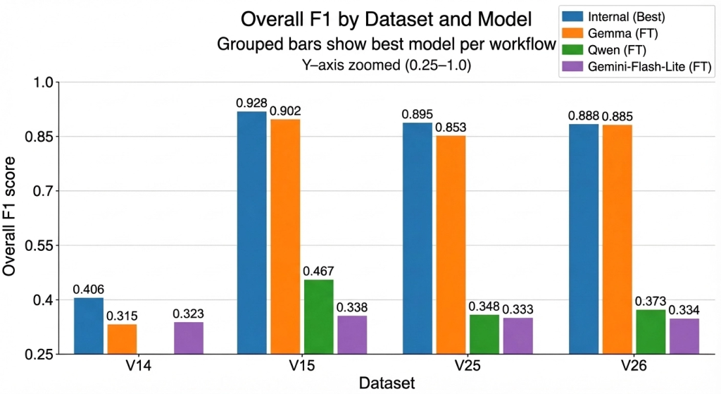
Final Showdown
After three rounds of experimentation, from the managed expressway to the hands-on workshop, the final results are in. The table below presents the single top-performing model from each workflow, providing a clear, “best-of-the-best” comparison that directly answers our core question.
Final ‘Best-of-the-Best’ Performance Summary
The Verdict: Lessons from the Race
So, can fine-tuned LLMs beat custom classifiers? Yes—but only if you have the right tools and the control to use them. The table above tells the whole story.
- Control is King. This was the single most important factor. The “Managed Expressway” (Gemini) was fast, but its “black box” nature locked us into a failing strategy. The “Custom Highway” (Gemma) gave us the control to diagnose and fix the core problem, leading to our breakthrough. Ultimate control (Qwen) offered deep insights but required more optimization. The clear lesson is that for complex tasks, you must have enough control to shape the architecture to your problem.
- Full Fine-Tuning vs. PEFT (LoRA): Power vs. Efficiency. Our experiment provides a clear picture of the trade-offs. The full fine-tuning approach with Gemma provided the raw power needed for the model’s weights to fully adapt to our nuanced task, ultimately delivering the winning performance. In contrast, the LoRA-based approach in the managed Gemini workflow was too constrained to succeed. However, our Qwen experiment showed that a transparent and controllable LoRA implementation (via
unsloth) is a highly efficient and viable option for resource-constrained environments, even if it doesn’t reach the absolute performance peak of full tuning without further optimization. The choice is a strategic one: seek maximum performance with full tuning, or opt for efficiency with a well-controlled PEFT approach. - Generative Models Need “Guardrails” for Classification. A standard LLM’s goal is to predict the next word, which causes it to favor the majority class in an imbalanced classification task. Our successful workflows show that you must implement “guardrails” to force a true discriminative choice. The
LogitsProcessorin our Gemma workflow and the trimmed classification head in the Qwen workflow are two different, powerful examples of such guardrails. - The “How” is More Important Than the “What.” Ultimately, our success was not about choosing “Gemma” over “Gemini.” It was about choosing a custom, controlled process over a managed one. A well-engineered pipeline on an open-weights model proved far superior to a less-controlled approach on a state-of-the-art model.
Disclaimer: This content was created with AI assistance. All research and conclusions are the work of the WPP AI Lab team.